
The 2022 National Assessment of Educational Progress (NAEP), also known as the Nation’s Report Card, has raised alarms across the country. Educators, policymakers, researchers, and parents are concerned about the results showing nationwide declines in both reading and math scores at both the 4th and 8th grade levels.
With such a troubling national outlook, it’s natural to look for bright spots—states or districts that bore up against the tidal wave of learning loss. In the context of large declines nationally, districts or states that held steady might reasonably be viewed as bright spots. But commentators get the story wrong if they interpret the absence of a statistically significant decline as an indicator of holding steady. As noted in our previous post, a nonsignificant difference does not mean there was no change—and some changes that are educationally meaningful may not achieve statistical significance.
Nonetheless, the limitations of statistical significance do not mean we can’t look for patterns and for bright spots. There is useful information in the state- and district-level NAEP results, if we use the right tools to extract it. Bayesian statistical analysis fits this bill. Unlike statistical significance testing, Bayesian methods incorporate contextual data—in this case, the wealth of results the National Center for Education Statistics (NCES) provides for each of four subject and grade-level combinations across all states and 26 urban school districts. The results improve our understanding of outcomes for any specific state or district (and each specific subject and grade level in that state or district).
Because Bayesian methods strengthen results and provide a more flexible framework for interpreting them, they provide more information than a judgment about whether a change was statistically significant. Bayesian analysis can tell us the likelihood that a change was educationally meaningful, as defined in terms of student learning. And it is far less likely to be misinterpreted than a judgment of statistical significance (or nonsignificance), because unlike statistical significance, a Bayesian result can be clearly stated in plain English, as we’ll show you in the paragraphs below.
The first step is to define what counts as educationally meaningful. The NCES commissioner has suggested that changes of only 1 or 2 points on the NAEP scale are educationally meaningful. For the purposes of this analysis, we set a slightly higher bar and define educationally meaningful as a 3-point change, which corresponds to just over a quarter of a year of learning, according to the Stanford Education Data Archive.
We re-analyzed the 2019 and 2022 average NAEP scores for subjects and grade levels at the state and district levels using Bayesian methods. The results, available in full at the bottom of this page, provide a clearer picture for individual districts and states, and stronger evidence about patterns across districts and states. The results illustrate the probability that each state and district experienced an increase or decline in its average score, and the probability that the increase or decline was educationally meaningful. (For those interested, the final tab in the figure describes more details about the methodology).
Let’s consider, for example, results for the District of Columbia Public Schools (DCPS), as shown in this figure.
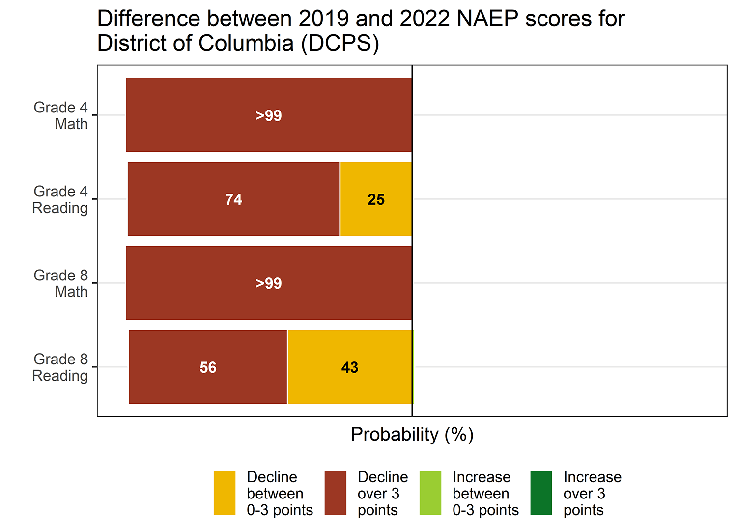
In math, declines in both grades in DCPS were unequivocal: NCES judged them to be statistically significant, and our Bayesian analysis also finds that the declines were substantial—virtually certain to be educationally meaningful: the red part of the bar indicates the probability of a decline exceeding 3 points.
In reading, the change in NAEP scores in DCPS was not statistically significant, according to the original results from NCES. But this does not mean that reading scores in DCPS “held steady,” as some stories reported. Bayesian analysis indicates that, rather than holding steady, DCPS 4th and 8th graders most likely lost ground in reading, as indicated by the collective probabilities in the red bar (probability of an educationally meaningful decline) and the orange bar (probability of a smaller decline). In fact, we estimate a 74 percent chance that DCPS 4th graders experienced an educationally meaningful decline in reading of 3 or more points, and a 25 percent chance of a decline smaller than 3 points. For DCPS 8th graders, we estimate a 56 percent chance that reading scores decreased by an educationally meaningful amount, and a 43 percent chance of a smaller decline.
The high probabilities of educationally meaningful declines in reading are consistent with the declines on DCPS’s scores on Partnership for Assessment of Readiness for College and Careers (PARCC) assessments, which are used for accountability in the District of Columbia and benefit from a more robust sample size than the NAEP. (As noted in our previous post, when sample sizes are small, meaningfully large differences may not be statistically significant.) But the NAEP results provide considerably more information than a simple assessment of statistical significance implies—if they are interpreted in a Bayesian framework.
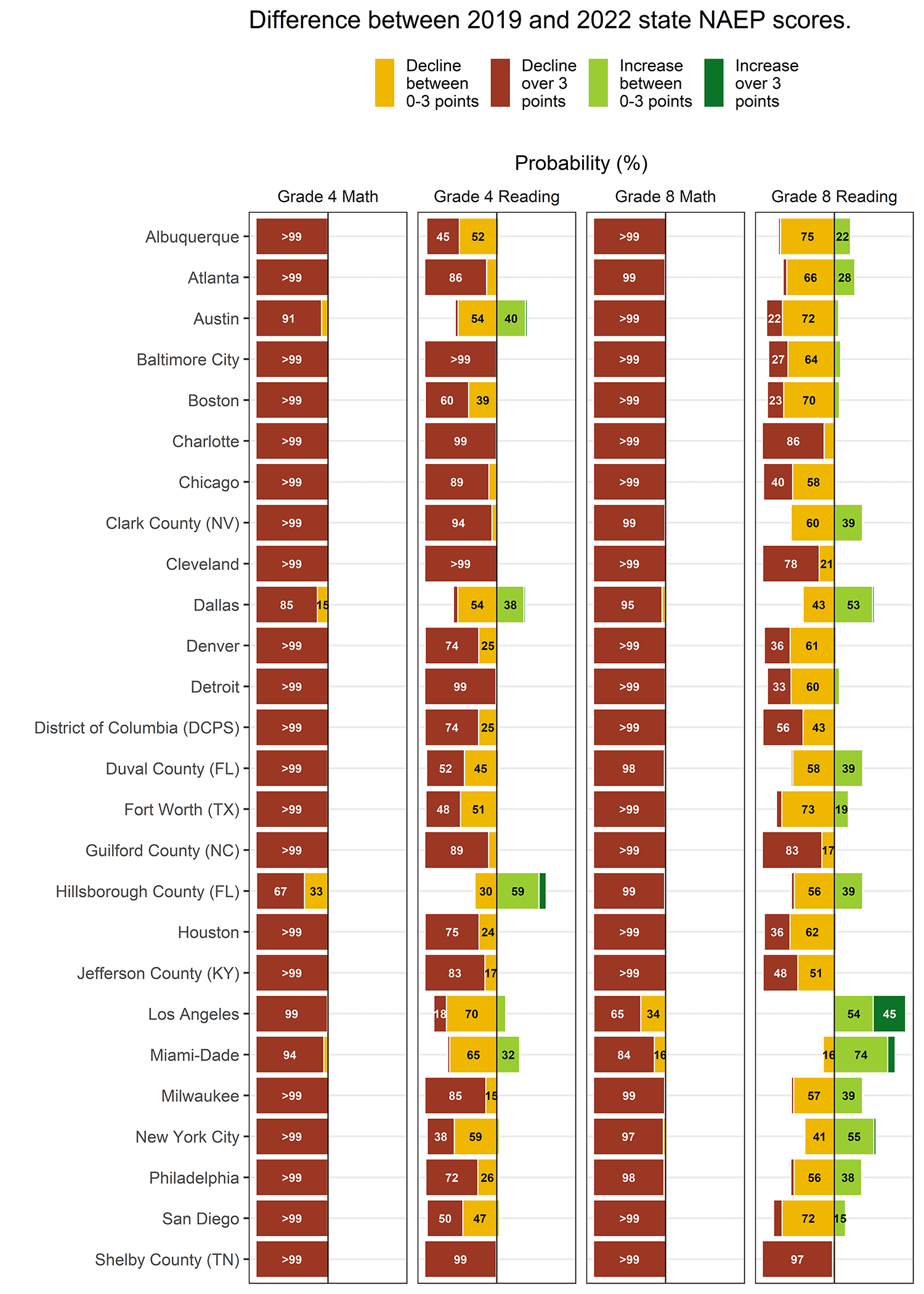
The richer information produced by a Bayesian interpretation comes into clearer focus when we summarize changes in NAEP scores across districts, as shown in the 'local' tab of the full results below. For each grade and subject the probability of declines appears to the left of the centerline, while increases appear to the right of it. The results show educationally meaningful changes (greater than 3 points), in red for declines and dark green for increases. Smaller changes (less than 3 points) appear in orange for declines and light green for increases.
A quick glance at these results confirms one pattern that emerged when scores were released: Declines were larger and more common in math than in reading.
But the Bayesian results also show that declines were more universal than much of the commentary has suggested. For example, NCES reported that 4th-grade reading scores declined by a statistically significant margin in 9 of 26 districts and did not change significantly in the remaining 17 districts. This is technically correct but easily misunderstood. Indeed, NCES communications encouraged the misinterpretation that 4th-grade reading scores “held steady” in these 17 districts.
In fact, the Bayesian analysis shows that that 4th-grade reading scores likely declined in 25 of 26 districts. Furthermore, declines were likely educationally meaningful in 17 of those districts.[1] This means that in 4th-grade reading, there was a meaningful educational decline in roughly half of the districts where changes were not statistically significant. And nearly all of these districts likely had at least a modest decline. The bottom line: There aren’t many bright spots here.
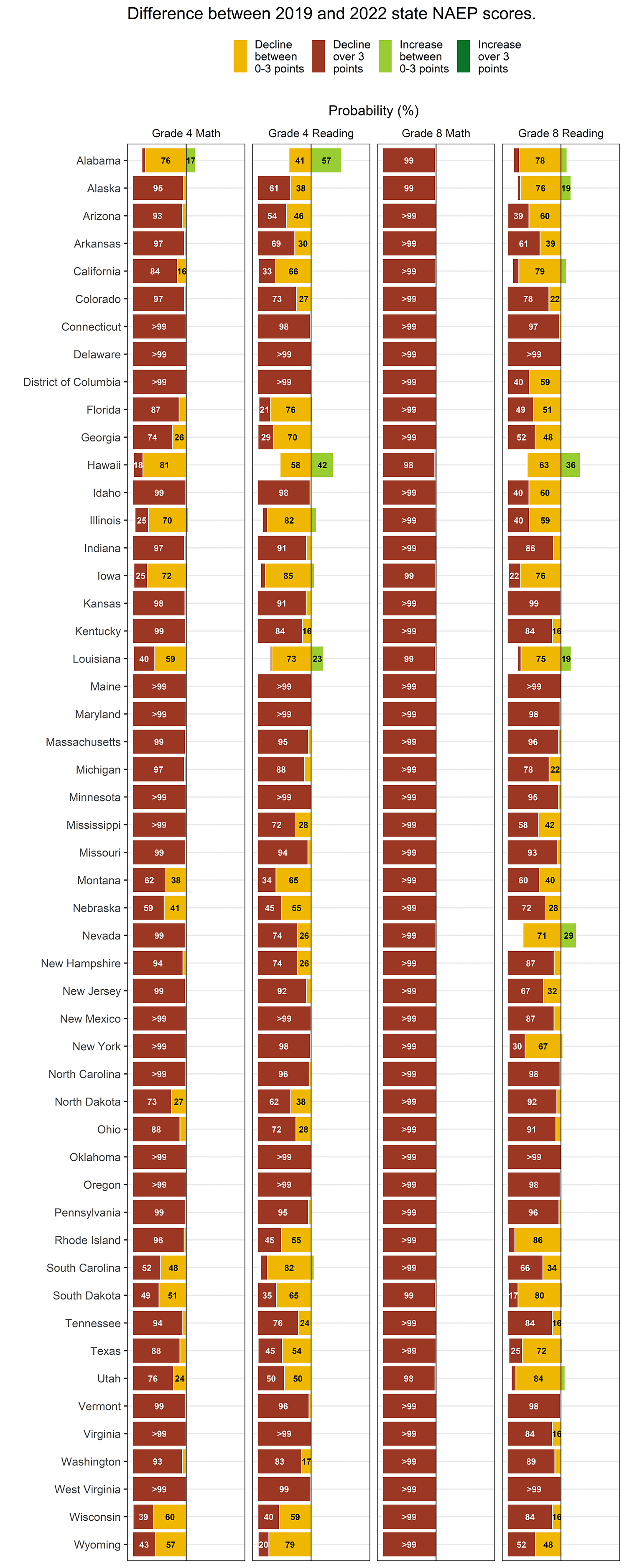
The counts of statistically significant and educationally meaningful declines diverge less at the state level than at the district level, as can be seen in comparing the Bayesian results on our state NAEP tab with the NCES reports of statistically significant declines. NAEP includes more students in state-level samples than district-level samples, making it more likely that an educationally meaningful decline will be statistically significant. But even so, the Bayesian results make clear that declines were much more common across the country than counts of statistically significant results would suggest.
More generally, a Bayesian interpretation provides more information about the true likelihood of changes and the size of those changes. As researchers, we owe it to journalists, policymakers, and the public to report findings in ways that reduce misunderstandings and make full, efficient use of the available information.
[1] It may occur to some readers that, to be consistent Bayesians, we shouldn’t count the number of individual districts with likely declines exceeding 3 points. Instead, we should construct a Bayesian estimate of the number likely to have declined more than 3 points, without regard to which specific districts met that threshold. A Bayesian estimate of the number might differ slightly from the count of districts with probabilities exceeding 50 percent. So we conducted this analysis to check. We found that the Bayesian estimates of the number differed from these counts by one in both cases: a fully Bayesian estimate suggests that 25 districts (rather than 26) likely experienced declines in 4th-grade reading, 16 of which (rather than 17) were educationally meaningful in size. For the other grades and subjects, fully Bayesian estimates of the number of districts and states with declines and educationally meaningful declines differed by no more than two districts or states from our counts of individual Bayesian estimates. Our general conclusions still hold.
Changes in average NAEP scores from 2019 to 2022
Our re-analysis fit two Bayesian models - one for states, and another for districts - that borrow strength across subjects, grades, and jurisdictions. Conforming with best practices in the literature, we we chose weakly informative prior distributions that assume that parameters governing variability should not be too large. We fit our models using Hamiltonian Monte Carlo as implemented in the Stan probabilistic programming language and assessed convergence and mixing using the Gelman-Rubin diagnostic and effective sample sizes.
Our models used imputed 2019 scores for Los Angeles, as Los Angeles excluded charter schools on a one-time basis in 2019 (which comprise nearly 20% of Los Angeles’ public schools).
Model specification
We write each of our Bayesian models as follows, where jurisdictions represent states or districts, respectively. Let \(j\) represent jurisdictions, \(s\) represent subject (Math or Reading), and \(g\) represent grade (fourth or eighth). Let \(t\) indicate academic year (2018/19 or 2021/22).
Then \(y_{jtsg}\) gives the NAEP score for jurisdiction \(j\) in year \(t\) for subject \(s\) in grade \(g\).
\[ y_{jtsg} = \alpha_{jsg} + \delta_{jsg}I_{\left\{t=2022\right\}} + \epsilon_{jtsg} \\ % % \alpha_{jsg} = \alpha_j^0 + \alpha_j^S S_s + \alpha_j^G G_g + \alpha_j^X S_s G_g \\ % \delta_{jsg} = \delta_j^0 + \delta_j^S S_s + \delta_j^G G_g + \delta_j^X S_s G_g \\ % \epsilon_{jtsg} \sim N(0, \sigma^2_{jtsg}) \] where standard errors \(\sigma_{jtsg}\) are specified using values from the NAEP data. In this parametrization, we let
- \(S_{Reading}=-0.5\)
- \(S_{Math}=0.5\)
- \(G_4=-0.5\)
- \(G_8=0.5\)
so that neither grade or subject is considered a baseline value. (Note that under this parametrization, the \(\alpha_j^0\) and \(\delta_j^0\) terms do not refer to a specific grade or subject, so are not directly interpretable.)
The eight random effects (four \(\alpha_{jsg}\)’s, and four \(\delta_{jsg}\)’s, for each subject-grade combination) are assigned prior distribution \(MVN(\theta_0,\Sigma)\), with an LKJ prior on \(\Sigma\). We transform the NAEP scores to z-scores prior to fitting the model and assign other parameters standard normal priors, reflecting a gentle assumption that these parameters are unlikely to be too large.
Model fitting and validation
We fit our model using Hamiltonian Monte Carlo as implemented in the Stan probablistic programming language (Stan Development Team, 2021), via its R interface, rstan. Specifically, we used the brms R package to implement our model using rstan.
We specified our brms model statement as follows, where y represented NAEP scores, y_se represented the corresponding standard errors, Y2022 is an indicator for the 2021/22 academic year, and grade_ctr and subj_ctr represent the \(S_s\) and \(G_g\) variables defined above.
We assessed convergence and mixing using the Gelman-Rubin diagnostic and effective sample sizes.
- For both our local and state models, Gelman-Rubin statistics were well within recommended ranges for all parameters (from 0.99 to 1.01 for both models).
- Effective sample sizes for all parameters were sufficient, with minimums of 838 for the local model and 506 for the state model.
Imputed scores for Los Angeles
Prior to fitting our models, we imputed two values for each subject-grade combination for Los Angeles in 2019 – the NAEP score, and its standard error.
- We imputed Los Angeles’ scores by calculating the percentile across districts that Los Angeles achieved in 2017 and assigning the corresponding 2019 percentile, separately by grade and subject.
- We used the same approach for standard errors, calculating the percentile of standard errors across districts for Los Angeles in 2017, ensuring that both the score itself and the level of precision reflect realistic scenarios based on Los Angeles’ 2017 performance.